An equation is simply a mathematical statement of equality. It says that two expressions are worth the same thing. But here is the catch. One or both sides might contain unknowns. These are the variables you need to solve for.
We use equations to untangle problems. They work in geometry. They work in chemistry. They handle physics too. And they matter in everyday life, not just in lab research.
Not every equation is a straight line to one answer. Some have no solution at all. Others have multiple answers. Some have just one. It depends on the problem you are trying to crack.
The Anatomy of an Equation
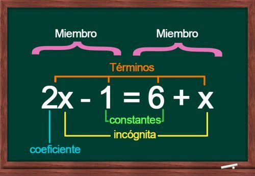
Every equation has two distinct parts. They are called members. You see them separated by that familiar equals sign (=).
Each member is built from terms. Think of terms as individual building blocks. These blocks are monomials.
What goes inside those monomials? It varies. You might find:
- Constants: fixed numbers that never change.
- Coefficients: numbers multiplying the variables.
- Variables: the letters representing unknown values.
- Functions: complex operations like sine or logarithms.
- Vectors: quantities with both magnitude and direction.
The unknowns themselves are usually letters. We use them as placeholders until we do the math to reveal their true value.
An equation is a balance scale. Whatever you do to one side, you must do to the other to keep it level.
Why does this structure matter? Because knowing the parts helps you tackle the whole. You can’t solve for X if you don’t recognize what X is attached to. Whether you are a student struggling with algebra or a parent helping with homework, breaking it down makes it less scary.
Start by identifying the members. Find the equals sign. Look at the terms on each side. Spot the variables. Once you see the structure, the solution often becomes clear. It is not magic. It is just logic arranged neatly.
And if you get stuck? That is normal. Even experts hit walls. The key is to look at one term at a time. Simplify. Rearrange. Keep the balance.
There is always more to unpack in equations. We have only scratched the surface here. The real work begins when you start applying these basics to harder problems.
How to classify equations by their mathematical structure
Understanding the skeleton of an equation changes how you solve it. You don’t just look for a variable; you look for the degree. The power to which the unknown is raised dictates the entire strategy.
Linear equations: the starting point
First-degree equations are the backbone of algebra. They are linear. This means the variable stands alone, raised to the power of one. There are no products between variables. No $x^2$. No $xy$.
The standard form is simple:
$ax + b = 0$
This is where most students begin. One variable. One slope. The solution is straightforward because the relationship is direct. If you double $x$, you double the result. This linearity makes these equations predictable and easy to isolate.
Quadratic equations: when things curve
Step up the power, and complexity follows. In second-degree equations, also known as quadratics, the unknown term is squared.
The structure looks like this:
$ax^2 + bx + c = 0$
This squared term introduces a curve. It means you aren’t dealing with a straight line anymore. You are dealing with a parabola. This changes the number of possible solutions. A linear equation gives one answer. A quadratic can give two. Or none. Or just one if the curve just touches the axis.
The presence of the $x^2$ term is what separates this from the simple linear cases. It requires the quadratic formula or factoring techniques to crack.
Cubic and higher-degree polynomials
Third-degree equations, or cubics, take the unknown to the power of three.
The pattern expands:
$ax^3 + bx^2 + cx + d = 0$
As the degree climbs, the algebra gets heavier. Fourth-degree equations introduce another layer: the coefficients $a, b, c,$ and $d$ belong to a specific number system, usually real numbers ($\mathbb{R}$) or complex numbers ($\mathbb{C}$).
The general form for a fourth-degree equation adds another term:
$ax^4 + bx^3 + cx^2 + dx + e = 0$
Why does this matter? Because higher-degree polynomials can wiggle more. They can cross the zero line multiple times. A fourth-degree equation can have up to four distinct real roots. The geometry becomes more intricate. The algebraic methods for solving them become significantly more tedious.
Transcendental equations: breaking algebraic rules
Not every equation fits into the polynomial box. Some require functions that cannot be resolved through standard algebraic operations alone. These are transcendental equations.
They include at least one non-algebraic function. Think trigonometric functions like sine or cosine. Or exponential functions like $e^x$. Or logarithms.
When you see an $x$ inside a sine function, you can’t just isolate it by moving terms around. You need numerical methods or graphical analysis. The solution isn’t always a neat integer. It might be an irrational number that requires approximation.
Functional, Integral, and Differential equations
The scope widens further when the unknown isn’t a single number, but a whole function.
In functional equations, the variable you are solving for is a function itself. You